Markov Decision Process
Introduction
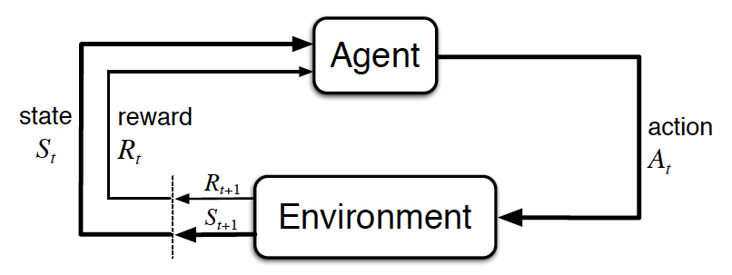
One of the most fundamental problems in reinforcement learning is the representation of the environment, which comprises everything that exists outside the agent. The agent interacts with the environment through actions, and the environment in turn responds to the agent with rewards and with new new situations, as shown in Figure 1.
A Markov decision process (MDP) provides a formal framework for modelling decision making, being a mathematically idealised instance of the reinforcement learning problem [1]. In this post we will explore the history of MDP, its definition, as well as some applications that can be formulated as MDPs.
Brief History
Markov decision processes were introduced by Richard Bellman as part of his research into solving the optimal control problem in the late 1950s. This problem deals with the design of a controller that optimises a measure of a dynamic system’s behaviour over a period of time. In that sense, MDPs are the discrete, stochastic version of the optimal control problem.
Bellman and others also developed an approach to find an “optimal return function” or value function, know today as the Bellman equation. The methods for solving the optimal control problem by solving the Bellman equation are known as dynamic programming. Later in the 1960s, Ronald Howard presented the policy iteration method for solving MPDs. The concepts described above form the foundation for modern reinforcement learning.
Definition
A Markov decision process is a tuple $(\mathrm{S}, \mathrm{A}, \mathrm{R})$ where:
- $\mathrm{S}$ is the state space set.
- $\mathrm{A}$ is the action space set.
- $\mathrm{R}$ is the reward space set.
The interaction between the agent and environment occurs in a sequence of time steps $t=0,1,2,3,\dots$. At each time step $t$, the agent receives a representation of the environment’s state $S_t \in S$, takes an action $A_t \in \mathrm{A}(s)$, receives a reward $R_{t+1} \in \mathrm{R} \subset \mathbb{R}$ and transitions to a new state $S_{t+1} \in S$.
This interaction causes a trajectory that begins as follows:
$$S_0, A_0, R_1, S_1, A_1, R_2, S_2, A_2, R_3, \dots$$
For finite MDPs, the sets in the tuple $(\mathrm{S}, \mathrm{A}, \mathrm{R})$ all have a finite number of elements, and the random variables $S_t$ and $R_t$ have well defined discrete probability distributions which depend only on the previous state and action. In other words, the probability of any given values $s' \in \mathrm{S}$ and $r \in \mathrm{R}$ occurring at time step $t$ is given by the values of the previous state and action. Formally:
$$P(s',r \mid s, a)\ \dot{=}\ \text{Pr}{S_t=s',R_t=r \mid S_{t-1}=s, A_{t-1}=a}$$
for all $s',s \in \mathrm{S}$, $r \in \mathrm{R}$, and $a \in \mathrm{A}$.
MDP framework
The MDP framework is abstract and can be applied in many different ways. Consider the following examples:
- Time steps need not be real time intervals, e.g. they can be sequence of steps in acting.
- Actions can be low-level, such as applying voltage to a robot’s actuator, or high level, such as navigating to a location.
- States can be determined by low-level sensations, such as direct sensor readings, or high level-representations, such as objects in a video frame.
In general, actions are any decisions we want to learn to make, and states are the information that is useful in making decisions. Moreover, the boundary between agent and environment is not the same as the boundary between a human, animal or robot’s body and the rest of the physical world. Instead, anything the agent has no control over is part of the environment.
Examples
Below are some examples of environments that can be represented by MDPs [2]:
| Environment | State space | Action space | Reward function |
|---|---|---|---|
| Hotter, colder: Guess a randomly selected number using hints |
Int range 0-3, where 0 means no guess yet submitted, 1 means guess is lower than the target, 2 means guess is equal to the target, and 3 means guess is higher than the target. |
Float from -2000.0 to 2000.0. The float is the number the agent is guessing. |
The reward is the squared percentage of the way the agent has guessed towards the target. |
| Cart Pole: Balance a pole in a cart |
A four-element vector with ranges from [-4.8, -Inf, -4.2, -Inf] to [4.8, Inf, 4.2, Inf]. First element is the cart position, second is the cart velocity, third is pole angle in radians, fourth is the pole velocity at tip. |
Int range 0-1. 0 means push cart left, 1 means push cart right. |
The reward is 1 for every step taken, including the terminal step |
| Lunar Lander: Navigate a lander to its landing pad |
An eight-element vector with ranges from [-Inf, -Inf, -Inf, -Inf, -Inf, -Inf, 0, 0] to [Inf, Inf, Inf, Inf, Inf, Inf, 1, 1]. First element is the x position, second the y position, the third is the x velocity, the fourth is the y velocity, fifth is the vehicle’s angle, sixth is the angular velocity, and the last two values are Booleans indicating legs contact with the ground. |
Int range 0-3. 0 means do nothing, 1 means fire left engine, 2 means fire main engine, 3 means fire right engine. |
The reward for landing is 200. There is a reward for moving from the top to the landing pad, for crashing or coming to rest, for each leg touching the ground, and for firing the engines. |
| Pong: Bounce the ball past the opponent, and avoid letting the ball pass you |
A tensor of shape [2021, 160, 3]. Values ranging 0-225. Represents a game screen image. |
Int range 0-5. Action 0 is do nothing, 1 is fire, 2 is up, 3 is right, 4 is left, 5 is down. Notice how some actions don’t affect the game in any way. In reality the paddle can only move up or down, or not move. |
The reward is 1 when the ball goes beyond the opponent, and a -1 when your agent’s paddle misses the ball. |
| Humanoid: Make a robot run as fast as possible and not fall |
A 44-element (or more, depending on the implementation) vector. Values ranging from -Inf to Inf. Represents the position and velocities of the robot’s joints. |
A 17-element vector. Values ranging from -Inf to Inf. Represents the forces to apply to the robot’s joints. |
The reward is calculated based on forward motion with a small penalty to encourage a natural gait. |
Note that for some environments, such as the cart pole one, obtaining the transition function can be achieved by looking at the code implementing the dynamics. For other environments, such as Pong, the dynamics are hidden inside an Atari emulator and the corresponding ROM file.
References
- Sutton, R.S. and Barto, A.G., 2018. Reinforcement learning: An introduction. MIT press.
- Morales, M., 2020. Grokking deep reinforcement learning. Simon and Schuster.